The Hopf fibration of $\mathbb{S}^3$ allows us to loosely describe the three sphere as being “a sphere’s worth of circles”. Stereographic projection and the complex numbers provide us a very useful window into the three-spherical world, so here we will go on a tour, trying to understand what this first sentence means through pictures.

Spherical Latitude

We will end up introducing the Hopf fibration as a way of building a toroidal coordinate system on the three sphere, so first let’s get comfortable with our new world by building a generalization of the familiar latitude and longitude system we use on $\mathbb{S}^2$.

To construct latitude and longitude, we start by picking a pair of antipodal points on the two-sphere and declaring one to be the “north pole” and the other the “south pole”. These points lie on an interval which passes through the center of the sphere, and slicing the sphere with planes perpendicular to this interval decomposes $\mathbb{S}^2$ into a union of two points and an intervals worth of circles of increasing, then decreasing radius.

Drawing an arc from the north pole to the south pole, we can label each of these circles with its “latitude”, or the angular distance from the north pole. To complete our coordinate system, we just need to take the standard angle coordinates on a circle and use them on each circular slice: latitude tells us which circle we are on, longitude tells us where on that circle, and we’re done!

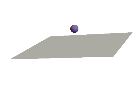
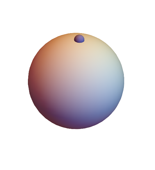
Now let’s try and do the same thing one dimension up. On the three-sphere, we can choose a pair of antipodal points and call them the north and south poles, and look at the slices perpendicular to the line joining these.  Of course, as everything is one dimension up, we are not slicing with planes but with three-dimensional subspaces, and our slices are not circles but 2-spheres. These spheres are the spheres of constant latitude, and they increase in size until reaching the equator (the sphere equidistant from our chosen antipodal points) and then collapse back down.

Slices of the 3-sphere by 3-planes orthogonal to the line connecting the north pole to the south pole.

We may assign each of these 2-spheres an angular coordinate telling us how far it is from the north pole, and then to specify our location on the 2-sphere we can use the standard spherical coordinates we built above. If we place the north pole at the projection point of stereographic projection, we can actually see what this coordinate system looks like in $\mathbb{R}^3$: the origin is the south pole, and it is surrounded by concentric 2-spheres.  Of course, the size of the 2-spheres actually increases for a while (towards the 3-sphere’s equator) and then decreases but this is badly distorted by stereographic projection so their images continue to grow in size filling out all of $\mathbb{R}^3$ (the really large ones actually represent small spheres around the north pole).

This coordinate system decomposes the three sphere into circles, but not in a nice continuous way. Each 2-sphere of constant latitude has two “bad points” on it for the coordinate system, its own north and south pole. These all fit together in a “bad circle” of points, connecting the north and south pole of the three sphere to each other.  But each point off this bad circle lies on a particular 2-sphere of constant latitude, and then on a circle of constant latitude on that sphere. Thus, in addition to the circle of bad points, given two angles in $[0,\pi)$, one for the 3-spherical latitude and one for the 2-spherical latitude we get a well-defined circle in $\mathbb{S}^3$. And so, we may think of the three sphere as being a “bad circle” together with a squares worth of circles of constant latitudes.

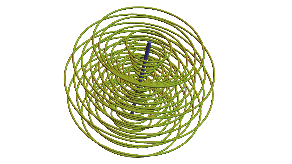
The blue line is the circle (through the projection point) of the north and south poles of each 2-sphere of constant latitude. The rest of $\mathbb{S}^3$ is filled with green circles.

Toroidal Latitude

While 3-spherical coordinates were rather natural for us to construct (via analogy to a lower dimensional case that we can actually see), they would not stand alone as the “obvious” coordinate system to an inhabitant of four dimensional space. Inside of four dimensional space we can choose a pair of orthogona planes, meeting at the origin in a single point. (If we were using the coordinates (x,y,z,w) these could be the xy and zw planes, for example). These planes intersect the three sphere in a pair of circles, which are linked with one another.

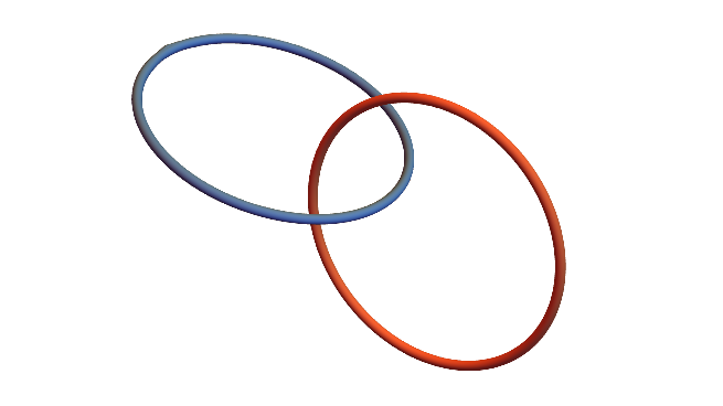
The two circles, viewed under stereographic projection with the projection point far from either circle.

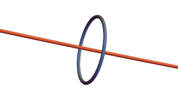
The same circles, viewed with the projection point on one of the circles. This will be our standard viewpoint.

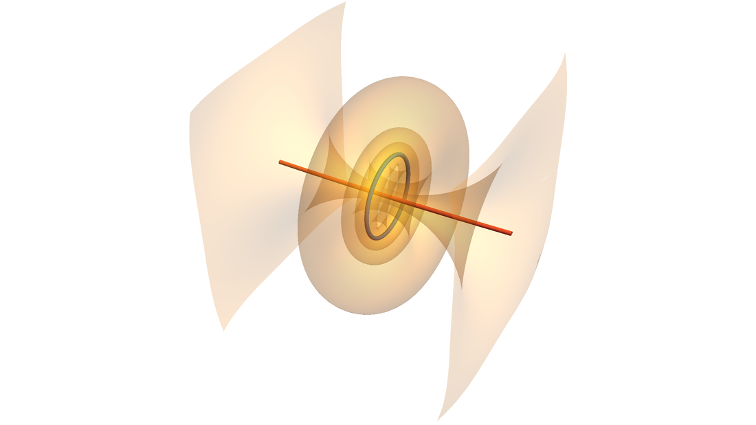
Now, lets call one of these circles the “north circle” and the other the “south circle”. In analogy to our earlier work we’d like to define the “surfaces of constant latitude” with respect to these pairs of circles. But whereas the surfaces equidistant from a point were spheres, the surfaces equidistant from a circle are tori!

Now, to complete our coordinate system on the three sphere, we just need to choose coordinates on a torus. And really, we just need to choose a way to decompose a torus into circles, as then we can just utilize the angle coordinate on a circle for our last coordinate. Below are two ways to do this:

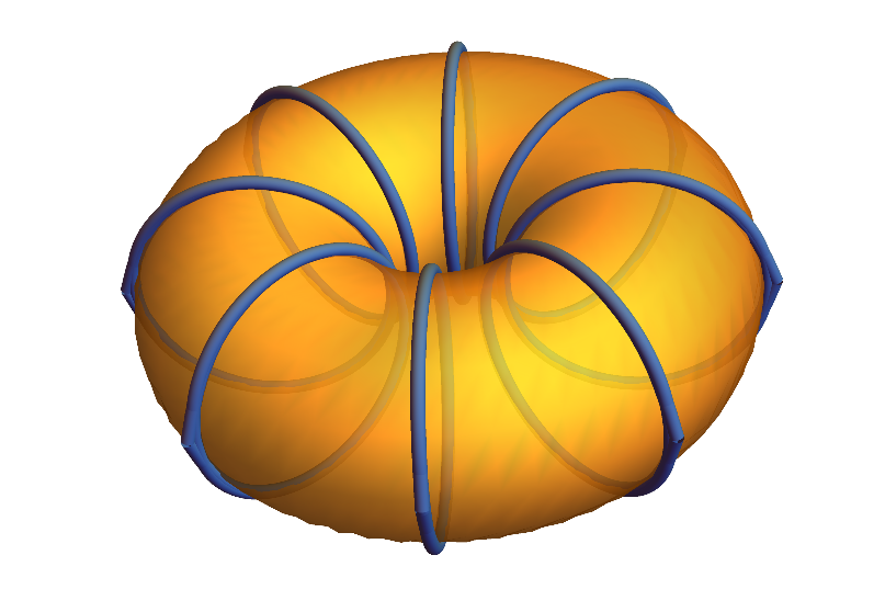
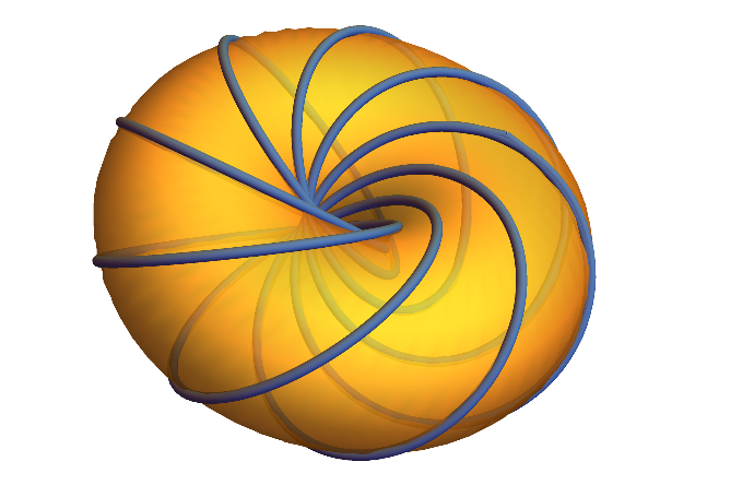
Both of these choices would lead to coordinate systems on the three sphere: after choosing a north and south circle, you specify on which torus of constant latitude you lie, and then on that torus you specify which circle, and then on that circle, which point. However, for our purposes here its only the second of the two options that interests us. Why?  Well lets look at what happens to our families of circles in each case as we approach the south circle: in the first case each of our circles shrinks to a point as the torus collapses onto the south circle, but in the second each circle lands neatly directly on the south circle itself.

Roughly, this shows that the north and south circles aren’t bad points of our coordinate system, as the north and south pole are in standard spherical coordinates, so this system is a bit more symmetric. In fact, this is just a hint as to how symmetric this collection of circles is - while it appears that we massively broke the symmetry of our original situation by choosing a north and south circle, it turns out we did not. In the final collection of circles, any pair of orthogonal circles whatsoever can be chosen and it turns out that the rest of the circles lie neatly on tori of constant latitude with respect to these. Of course, this is far from obvious given the construction we just gave. To see this, we will start over and look at another process leading to the same collection of circles: looking at point preimages under the Hopf map.

One final note before moving on though: just like standard spherical coordinates extended to let us think of the 3-sphere as an intervals worth of spheres or as a circle together with a squares worth of additional circles, we might ask ourselves what the space of circles looks like here. Well, on each torus of constant latitude there is a circles worth of circles; and there’s an interval worth of tori so this gives us a cylinder’s worth of circles. Together with a point for the north circle and a point for the south circle, these fit together to form a sphere.

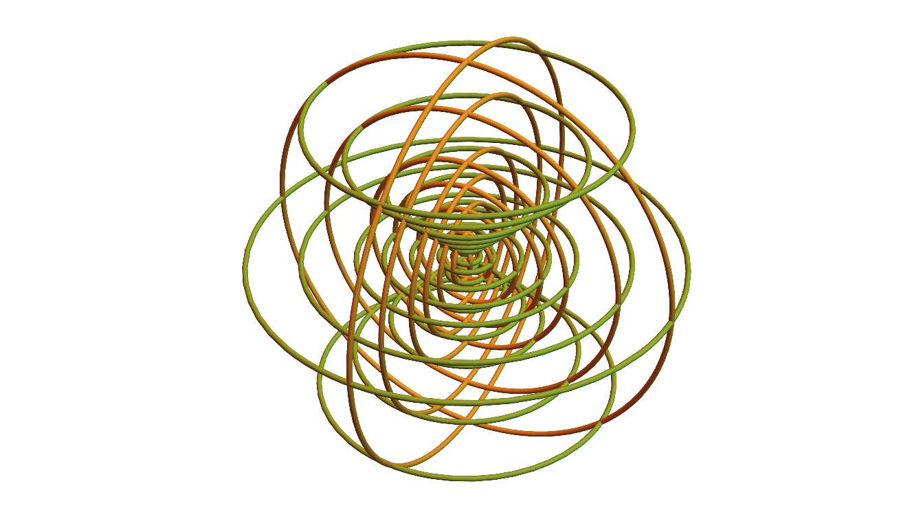
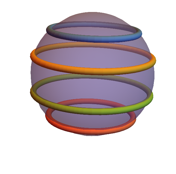
Below we see a collection of circles in the three sphere lying on tori of constant latitudes, and the corresponding circles on the 2-sphere.

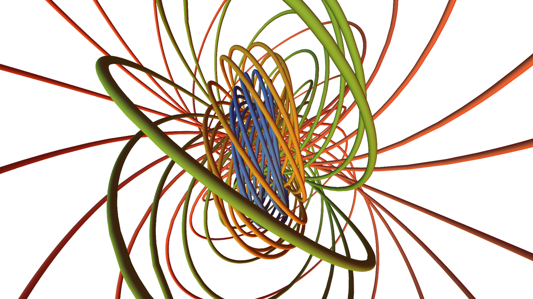
Thus, this coordinate system decomposes the 3-sphere into a 2-sphere’s worth of 1-spheres! Now that’s pretty beautiful!

Complex Subspaces

Ok, bear with me for a minute while we go on a seemingly unrelated tangent. Being even dimensional, we can think of four dimensional space as either a product of four copies of $\mathbb{R}$ or two copies of $\mathbb{C}$. To fix notation, we will denote a point in four dimensional space in one of the following ways:

$$\mathbb{R}^4\ni (a,b,c,d)\cong (a+bi,c+di)=(z,w)\in\mathbb{C}^2$$

Thought of over the reals, every plane through the origin is a 2-dimensional vector subspace, but this is not true when thought of as a vector space over $\mathbb{C}$. For instance, the plane ${(a,0,c,0) : a,c,\in\mathbb{R}}$ is not a complex 1-dimensional subspace of $\mathbb{C}^2$ as it is not the (complex) span of any single vector. It turns out we can quantify this difference precisely: the set of real 2-dimensional subspaces of $\mathbb{R}^4$ is a four dimensional manifold ($\mathbb{Gr}(4,2)$), but the set of complex planes in $\mathbb{C}^2$ is two dimensional ($\mathbb{C}\textrm{P}^1$).

Let’s think a bit more about the structure of the space of complex subspaces of $\mathbb{C}^2$. First of all, the union of all of them is clearly $\mathbb{C}^2$ as given any $\vec{v}\in\mathbb{C}^2$ we have the complex subspace $\textrm{span}_\mathbb{C}(\vec{v})$. But furthermore this union is almost disjoint: two complex subspaces only intersect in the origin! (Remember, they only have one complex dimension so if they share a nonzero vector they are equal). Intersecting any plane through the origin with the three-sphere gives a great circle, and so the collection of complex subspaces of $\mathbb{C}^2$ gives rise to a collection of circles in $\mathbb{S}^3$.  And by the discussion above, we can see that this collection of circles are pairwise disjoint and union to all of $\mathbb{S}^3$.

This collection of circles in $\mathbb{S}^3$ is incredibly symmetric. For example, choose any two pairs of circles from the collection: each pair represents a pair of distinct 1-dimensional subspaces of $\mathbb{C}^2$, and so choosing a vector from each, gives a basis for $\mathbb{C}^2$. But clearly there is a linear transformation taking one of these bases to the other, and after a little thinking this gives us a homeomorphism of $\mathbb{S}^3$ taking any pair of circles to any other pair of circles. In particular, note that in the coordinates $(z,w)$ on $\mathbb{C}^2$ the planes $z=0$ and $w=0$ give rise to the “north circle” and “south circle” we discussed previously, and so there is a homeomorphism taking any pair of circles to the north-south pair. Thus, every pair of circles are linked just like these two!

Thus, this gives us a way to decompose the three sphere into a union of disjoint circles, which is symmetric enough that each pair of circles looks like every other pair.
This family is parameterized by the space of complex subspaces of $\mathbb{C}^2$, usually denoted as $\mathbb{C}\textrm{P}^1$. What does this space look like? Well, as each complex subspace of $\mathbb{C}^2$ can be thought of as simply an equivalence class of vectors under complex scalar multiplication (after ignoring $0$), we can coordinatize $\mathbb{C}\textrm{P}^1$ as

$$\mathbb{C}\textrm{P}^1=\frac{\mathbb{C}^2\smallsetminus{0}}{{\vec{v}\simeq \lambda \vec{v}: \lambda\in\mathbb{C}^\times}}$$

The standard notation is to denote the equivalence class of a point $(z,w)$ by $[z:w]$, and the relation by the equalities $[z:w]=[\lambda z: \lambda w]$. So, what does $\mathbb{C}\textrm{P}^1$ look like?  The plane $w=0$ is represented by the point $[1:0]$ (equivalently, $[z:0]$ for any $z\in\mathbb{C}^\times$), and if $w\neq 0$ then we have the equality

$$[z:w]=\left[\frac{1}{w} z:\frac{1}{w}w\right]=[\xi:1]$$

Where $\xi\in\mathbb{C}$ is uniquely determined for each plane. And so, $\mathbb{C}\textrm{P}^1$ looks like a copy of $\mathbb{C}$ together with a single point at infinity, which closes it up to make a 2-sphere.

This means that the collection of complex planes of $\mathbb{C}^2$ divides the three sphere into a sphere’s worth of circles, each pairwise linked! No surprise, this is the same collection of circles we came to above by considering a toroidal coordinate system. But now we have a precise way to write it all down, so let’s get to drawing pictures!

The Hopf Fibration

The projection map $\mathbb{C}^2\to \mathbb{C}\texrm{P}^1$ which takes each complex line to its associated point has the simple description $(z,w)\mapsto [z:w]$. When restricted to the three-sphere inside of $\mathbb{C}^2$ and with $\mathbb{C}\textrm{P}^1$ suitably interpreted as the two-sphere, this map is called the hopf map $h:\mathbb{S}^3\to\mathbb{S}^2$.  To illustrate this, I will draw the three sphere under stereographic projection, and draw a point on the two sphere for each circle in $\mathbb{S}^3$.

But even better than a picture is a video: as a point bounces around on $\mathbb{S}^2$, what happens to the associated circle in $\mathbb{S}^3$?. Lines of constant latitude on $\mathbb{S}^2$ correspond to circles worth of circles, or tori of constant latitude in $\mathbb{S^3}$. And these tori continuously fill the space between the pair of chosen circles concentrically (the following video only shows slices of each torus, otherwise you wouldn’t be able to see anything!

Here’s a more random collection of points on the two sphere and their associated circles: remember all pairs of circles are topologically equivalent and so the extra symmetry we saw above depending on us choosing a north and south circle was an artifact of our choices, not an intrinsic property of the fibration!